User Guide
Getting Started
It doesn’t take much to get nbstata up and running. Here’s how:
Prerequisites
Stata
Because nbstata uses pystata under the hood, a currently-licensed version of Stata 17+ must already be installed. (If you have an older version of Stata, consider stata_kernel instead.)
Make sure that the stata command (that is, the CLI to Stata, not to be confused with xstata, which is the GUI) works, otherwise nbstata won’t work.
In particular, if you are on Arch Linux and you get this error when running stata:
stata: error while loading shared libraries: libncurses.so.5: cannot open shared object file: No such file or directoryYou need to install ncurses5-compat-libs from the AUR to fix it.
Python
In order to install the kernel, you will also need Python 3.10 or higher.
- Stata 17 users can run nbstata under Python 3.10, 3.11, 3.12, and 3.13 but not under Python 3.14.
- Stata 18, 18.5, 19, and 19.5 users can run nbstata under Python 3.10, 3.11, 3.12, 3.13, and 3.14. For Python 3.14, users need to update their version of Stata to the 12 November 2025 revision (or later). To see your version of Stata’s revision date issue in Stata, run either
aboutordisplay c(born_date).
If are new to Python, I suggest installing the Anaconda distribution. This doesn’t require administrator privileges and is the simplest way to install Python, JupyterLab and many of the most popular scientific packages.
(However, the full Anaconda installation is quite large, and it includes many libraries for Python that nbstata doesn’t use. If you don’t plan to use Python and want to use less disk space, install Miniconda, a bare-bones version of Anaconda. Then, at an Anaconda prompt, type conda install jupyterlab to install JupyterLab.)
The remainder of this guide assumes you have a Anaconda installed, but all you really need is Python and JupyterLab (or some other way of making use of the Stata kernel, such as Quarto).
Install nbstata
To download and install the python package run the following at an Anaconda prompt:
pip install nbstataNext run the Stata kernel install script, which has the following syntax (with square brackets denoting options):
python -m nbstata.install [--sys-prefix] [--prefix PREFIX] [--conf-file]That is, the most basic kernel install command is just python -m nbstata.install. The options are explained in the next section.
Kernel setup options
Include --sys-prefix to install the kernel to sys.prefix (e.g. a virtualenv or conda env), or --prefix PREFIX if you want to specify the install path yourself (typing it in place of PREFIX).
The --conf-file option creates a configuration file for you. (Note: A configuration file will always be created if the installer cannot locate your Stata installation.)
The location of the configuration file will be:
[sys.prefix]/etc/nbstata.confif--sys-prefixor--prefixis specified.~/.config/nbstata/nbstata.confotherwise.
(If a configuration file exists in both locations at kernel runtime, the home directory (~) version takes precedence. For backwards compatibility, config files saved to ~/.nbstata.conf also work. When in doubt, the %status magic indicates the location of the operative config file.)
Updating
To upgrade from a previous version of nbstata, run:
pip install nbstata --upgradeWhen updating, you don’t have to run python -m nbstata.install again.
Configuration (optional)
The following settings are permitted inside the configuration file. Aside from the first three, they may also be set within your notebook using the %set magic explained below):
stata_dir: Stata installation directory.edition: Stata edition. Acceptable values are ‘be’, ‘se’ and ‘mp’. Default is ‘be’.splash: controls display of the splash message during Stata startup. Default is ‘False’.graph_format: Acceptable values are ‘png’ (the default), ‘pdf’, ‘svg’ and ‘pystata’. Specify the last option if you want to usepystata’s default setting.graph_width/graph_height: By default, graphs are generated with width 5.5in and height 4in. The width or height may be specified as a number (interpreted as inches) or a number and its unit (in, cm, or px). So3and3inare equivalent. Other valid examples:300pxand7.2 cm. (Note: These values may also be set todefault, which values alone enable thexsizeandysizeoptions on Stata graph commands to influence the graph output size. Any values other thandefaultoverride thexsizeandysizeoptions.)echo: controls the echo of commands, with the default being ‘None’:- ‘True’: echo all commands.
- ‘False’: for Stata 18.5+, not echo any command (native Stata implementation); otherwise echo only multi-line commands.
- ‘None’: not echo any command (custom nbstata implementation).
missing: What to display for a missing value in the output of the%browse,%head, and%tailmagics. Default is ‘.’, following Stata. To defer to pandas’s format forNaN, specify ‘pandas’.browse_auto_height: Whether to set ‘height: 100%’ for the %browse widget (default: ‘True’):- ‘True’: allows browse widget to expand to height of its container, such as when using ‘Create New View for Output’ in Jupyter Lab.
- ‘False’: fixed height of around 22 rows, recommended for NBClassic and VSCode.
Settings must be under the title [nbstata]. Not all settings need be included. Example:
[nbstata]
stata_dir = /opt/stata
splash = True
graph_format = pystata
graph_width = default
graph_height = default
echo = False
Default Graph Format
Both pystata and stata_kernel default to the SVG image format. nbstata (like pystata-kernel) defaults to the PNG image format instead for several reasons:
Syntax highlighting (Optional)
Stata syntax highlighting can be installed for Jupyter Lab:
pip install jupyterlab_stata_highlight2(If you prefer the standard Jupyter color scheme, the original jupyterlab-stata-highlight also works.)
Starting JupyterLab
You can start JupyterLab from within Anaconda Navigator. Or start it from an Anaconda prompt by running:
jupyter labEither should open it up in a new browser tab. From there, you can create a new Stata notebook.
Note: By default, you can only open/save notebooks within the directory from which JupyterLab is run. To access a different directory, you can instead start it up by running:
jupyter lab --notebook-dir "YOUR_PATH_HERE"Magics
‘Magics’ are commands provided by nbstata that enhance the experience of working with Stata in Jupyter. They work only when placed at the beginning of a code cell.
Jupyter magics typically start with %, but nbstata magics may alternatively be prefixed with *% so that, if you export a Stata notebook to a .do file and run it that way, the magics will not cause errors.
nbstata currently supports the following magics:
| Magic | Description | Full Syntax |
|---|---|---|
| %browse | Interactively view dataset | %browse [-h] [varlist] [if] [in] [, nolabel noformat] |
| %head | View first 5 (or N) rows | %head [-h] [N] [varlist] [if] [, nolabel noformat] |
| %tail | View last 5 (or N) rows | %tail [-h] [N] [varlist] [if] [, nolabel noformat] |
| %frbrowse | Interactively view frame | %frbrowse [-h] framename[: [varlist] [if] [in] [, nolabel noformat]] |
| %frhead | View first 5 (or N) frame rows | %frhead [-h] framename[: [N] [varlist] [if] [, nolabel noformat]] |
| %frtail | View last 5 (or N) frame rows | %frtail [-h] framename[: [N] [varlist] [if] [, nolabel noformat]] |
| %locals | List locals with their values | %locals |
| %delimit | Print the current delimiter | %delimit |
| %help | Display Stata help | %help [-h] command_or_topic_name |
| %set | Set single config option | %set [-h] key = value |
| %%set | Set multiple config options | %%set [-h] |
| %status | Display Stata/config status | %status |
| %%echo | Ensure echo from cell | %%echo |
| %%noecho | Suppress echo from cell | %%noecho |
| %%quietly | Suppress all output from cell | %%quietly |
You can run any magic with the -h option (--help) to see brief help documentation for the magic.
%browse, %head, %tail (and frame equivalents)
Quickly view your data
*%browse [-h] [varlist] [if] [in] [, nolabel noformat]
*%head [-h] [N] [varlist] [if] [, nolabel noformat]
*%tail [-h] [N] [varlist] [if] [, nolabel noformat]
These magics provide alternatives to Stata’s browse command, which is not available in a Stata notebook. They can each be called with standard Stata varlist and if syntax. %browse also supports Stata’s in syntax, whereas %head (and %tail), modeled after pandas, display the first (or last) 5 (or N) observations that meet the (optional) if criteria.
By default, the %browse, %head, and %tail magics convert numeric Stata values to strings using their Stata format and value labels. To prevent this behavior, specify the noformat and/or nolabel options.
The output of any of these, but especially that of %browse, may be expanded into a separate Jupyter Lab tab by right clicking it and selecting “Create New View for Output.”
%frbrowse, %frhead, and %frtail do the same for a frame specified as a prefix. Examples:
%frbrowse alt_frame
%frhead alt_frame: if var1 == 1, nolabels
%locals
List local macro names and values
This takes no arguments. The output format mimics Stata’s macro list command (which only displays global macros).
%delimit
Print the current Stata command delimiter
This takes no arguments; it prints the delimiter currently set: either cr or ;. If you want to change the delimiter, use #delimit ; or #delimit cr. The delimiter will remain set until changed.
[1]: %delimit
Current Stata command delimiter: cr
[2]: #delimit ;
delimiter now ;
[3]: *%delimit
Current Stata command delimiter: ;
[4]: #delimit cr
delimiter now cr
%help
Display a help file in rich text
*%help [-h] command_or_topic_nameAdd the term you want to search for after %help. For example:

The underlined terms in the output are links. Click on them to open further help in a new tab.
%set, %%set
Set configuration values
Usage:
*%set [-h] key = value*%%set
key1 = value1
[key2 = value2]
[...]key: Configuration setting name:graph_format,graph_width,graph_height,echo, ormissingvalue: Value to set. See Configuration above for more information.
Examples:
*%set graph_format = svg%%set
echo = True
missing = N/ATo prevent the cell magic %%set from causing an error if you export the notebook to a .do file and run it that way, you may surround the key-value statements with /* and */ on separate lines, like this:
*%%set
/*
echo = True
missing = N/A
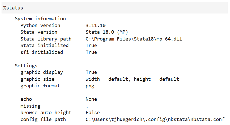
*/%status
Display Stata status and configuration values
%%echo %%noecho, %%quietly
Toggle cell output type
Putting %%echo at the top of a cell sets the configuration option echo = True for just that cell. For example, suppose you have configured echo = None but you do want to see the Stata commands echoed for a particular cell:
[1]: *%%echo
     disp 1
     disp 2
. disp 1
1

. disp 2
2

.
Similarly, %%noecho sets the configuration option echo = None for a single cell:
[2]: *%%noecho
     disp 1
     disp 2
1
2
%%quietly silences all cell output, including graphs. It is a convenience magic equivalent to placing the standard Stata code quietly { at the start and } at the end of the cell.
[3]: *%%quietly
     disp 1
     disp 2
Stata Implementation Details
#delimit behavior
A #delimit; command in one cell will persist into other cells, until #delimit cr is called. For example, see delimit tests.ipynb.
echo = None: potential for unanticipated errors
With Stata 18.5+, echo = False is recommended.
The default echo = None configuration does some complicated things under the hood to emulate functionality that pystata does not directly support: running multi-line Stata code without echoing the commands. While extensive automatic tests are in place to help ensure its reliability, unanticipated issues may arise. If, while using this mode, a particular code cell is not working as expected, try placing the %%echo magic at the top of it to see if that resolves the issue. (If so, please report that here.) You can also avoid such potential issues by setting the config echo = False, which will at least not echo single-line Stata commands though it will echo multiple commands for Stata 17 and 18.0.
more and pause
Stata’s more and pause commands do not work in a notebook, so these features should remain in their default ‘off’ states (i.e., set more off and pause off).
linesize
Unlike in the official Stata interface, the width of Stata output will not automatically adjust to the width of your window. Instead, you can use the set linesize Stata command to change it manually. For example:
set linesize 130Quarto tips
nbstata can be used with Quarto, starting from either a notebook or a .qmd markdown file, to create output in a wide variety of formats. Just include jupyter: nbstata in the document-level YAML at the top and use *| as the prefix for cell options.
Inline calculations
With nbstata v0.8+, you can use the standard Quarto syntax for inline code, specifying the Stata expression as ‘[%fmt] exp’, just as you would for a Stata display command. For example:
```{stata}
*| include: False
sysuse auto, clear
regress price mpg
```
An *increase* of one mpg is associated with a *decrease* in price of \$`{stata} %5.2f abs(_b[mpg])`.
would result in output like this:
An increase of one mpg is associated with a decrease in price of $238.89.
Stata locals cannot be referenced within inline code like `x’ because the tick (or “left single quote,” as Stata’s manual calls it) conflicts with Quarto’s inline code syntax. You can instead use globals or scalars to pass things to inline code.
For example, this gives the same output as above (whereas defining ‘mpg_coef’ as a local would not work):
```{stata}
*| include: False
scalar mpg_coef = string(abs(_b[mpg]), "%5.2f")
```
An *increase* of one mpg is associated with a *decrease* in price of \$`{stata} mpg_coef`.